Sinc interpolation
I've started reading more about Digital Signal Processing (DSP) techniques for use in the G4-Scope and find it all absolutely fascinating. Apart from numerous searches and articles on the web, the book which really drives things home for me is "Digital Signal Processing, A Practical Guide for Engineers and Scientists" by Steven K. Smith (2003).
Discrete signals, linear systems, impulse responses, convolutions, Fourier transforms, filter kernels, ... there sure is a lot of information (and math) out there to wade through.
Filing in the gaps
The goal I'm after, is to plot a signal trace on the scope screen when fewer samples are available than fit on the horizontal axis. When the steps are small enough, say at most 4 pixels between each sample in both horizontal and vertical directions, then drawing straignt lines should be fine. But when you have only one or two samples per division (25 pixels), this starts to look really bad. And yet it's not really about looks ... those sharp corners will suggest that there is much more detail than what the ADC could actually see!
For proper sampling at 5 MHz, any signal fed to the ADC needs to exclude all frequencies above 2.5 MHz. This is the Nyquist frequency. Anything higher leads to alisasing artifacts: signal effects showing up which are not actually present.
But the flip side of this limitation, is that a properly filtered input signal is also known to have bounded rise and fall times. As all DSP texts will point out, you only need two samples per signal cycles to fully reconstruct it, if no higher frequency is present. Take two samples, and only a single unique sine wave can be fitted through them.
The "sinc" function
And that's where the "sinc" function fits in. It's defined as sin(x) / x for
all x except when it is zero (then the value is defined as 1.0). Here are two
super-imposed plots:

(this image is from Wikipedia)

The blue plot is simply scaled differently (π•x iso x). It has as benefit
that it crosses the X-axis whenever x has an integer value.
The sinc function extends indefinitely on both sides, which prevents practical use. But it also quickly drops off, so ignoring both tails has only a minor impact on computational accuracy.
So what's the point of sinc?
Well, it turns out that it provides just the right coefficients to perform a weighted average over a few surrounding samples to produce a smooth interpolation between those samples. With "smooth" meaning: mathematically optimal filtering of properly anti-aliased ADC samples (and "weighted average" is just another way of saying ... convolution).
Think of it as being somewhat like smooth Bézier curves, except that it's not about looking good but about properly interpreting given samples ... and it also happens to look good.
There is some computation involved to create such a reconstructed signal, i.e. to produce results for the gaps between the sampled values: some sine function calls, and a few floating point multiplies and adds. But it's well worth it: the results are quite astonishing.
Duchon and Lanczos
The sinc function extends infinitely to both sides, but the coefficients it produces quickly reduce in magnitude. With a window function, the effects of truncation are limited. Without claiming to understand any of this, I decided to use Lanczos resampling for this. Wikipedia:
The filter was invented by Claude Duchon, who named it after Cornelius Lanczos due to Duchon's use of the sigma approximation in constructing the filter, a technique created by Lanczos.
With a crude from-scratch implementation in C++, it's easy to see what this all leads to:
- Generate 60 points of one complete sine wave, i.e. 6° apart.
- Sample it every 13 points, i.e. every 78° (intentionally not a pure fraction.
- Apply the sinc interpolation algorithm, with a Lanczos window of M=2.
- Visualise the result using Matplotlib in Python.
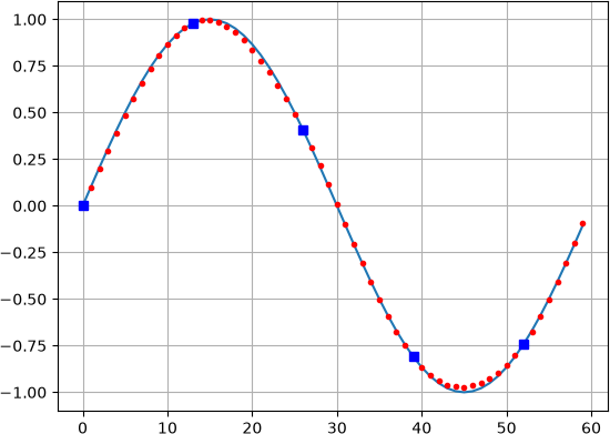
Here are all interpolated values between samples, on top of the original sine wave:
Just to make it clear: this interpolation has no knowledge that the input signal was a sine wave! All it assumes is that the input signal was bandwidth-limited, i.e. there are no frequencies above half the sample rate (yep ... there's that Nyquist fellow again).
As you can see in this plot, the interpolation is stunningly accurate, including overshoot past the highest and lowest sample values.
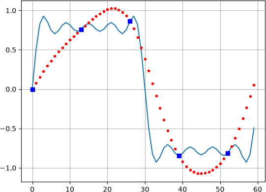
Here is what happens to interpolation when the input signal contains frequencies above the Nyquist limit:
This is the same sine wave, plus its 3rd, 5th, 7th, and 9th harmonic, i.e. the first 4 harmonics present in a square wave signal.
The interpolation still looks smooth (and passes through all sample points by design), but it is not able to track the changes produced by these higher frequencies. Or more accurately: there is not enough information in the samples - properly filtered, this interpolation would have been accurate.
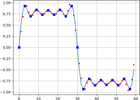
By sampling more often (every 3 points instead of every 13), the Nyquist frequency limit goes up. Now such a signal is more or less suitable for the higher sampling rate, and the result more closely matches what came in.
Or, to put it differently: that's how a 10x bandwidth scope can "see" square waves!